PPT LAB 3 Enzyme PowerPoint Presentation, free download ID4526880
Lineweaver-Burk analysis is one method of linearizing substrate-velocity data so as to determine the kinetic constants Km and Vmax. One creates a secondary, reciprocal plot: 1/velocity vs. 1/ [substrate].

LineweaverBurk plot for determining of K M and V max (casein as... Download Scientific Diagram
Moof's Medical Biochemistry Video Course: http://moof-university.thinkific.com/courses/medical-biochemistry-for-usmle-step-1-examFor Related Practice Problem.

(A) LineweaverBurk plot for the inhibition of eeAChE(A) and eqBChE (B)... Download Scientific
The Lineweaver-Burk plot allows us to determine the Vmax and Km values of an enzyme. Vmax represents the maximum velocity of the reaction, while Km represents the substrate concentration at which the reaction velocity is half of Vmax. These parameters provide valuable insights into the enzyme's efficiency and affinity for its substrate.

LineweaverBurk secondary plot for Ki calculation Download Scientific Diagram
For this mechanism, Lineweaver-Burk plots at varying A and different fixed values of B give a series of parallel lines. An example of this type of reaction might be low molecular weight protein tyrosine phosphatase against the small substrate p-initrophenylphosphate (A) which binds to the enzyme covalently with the expulsion of the product P.
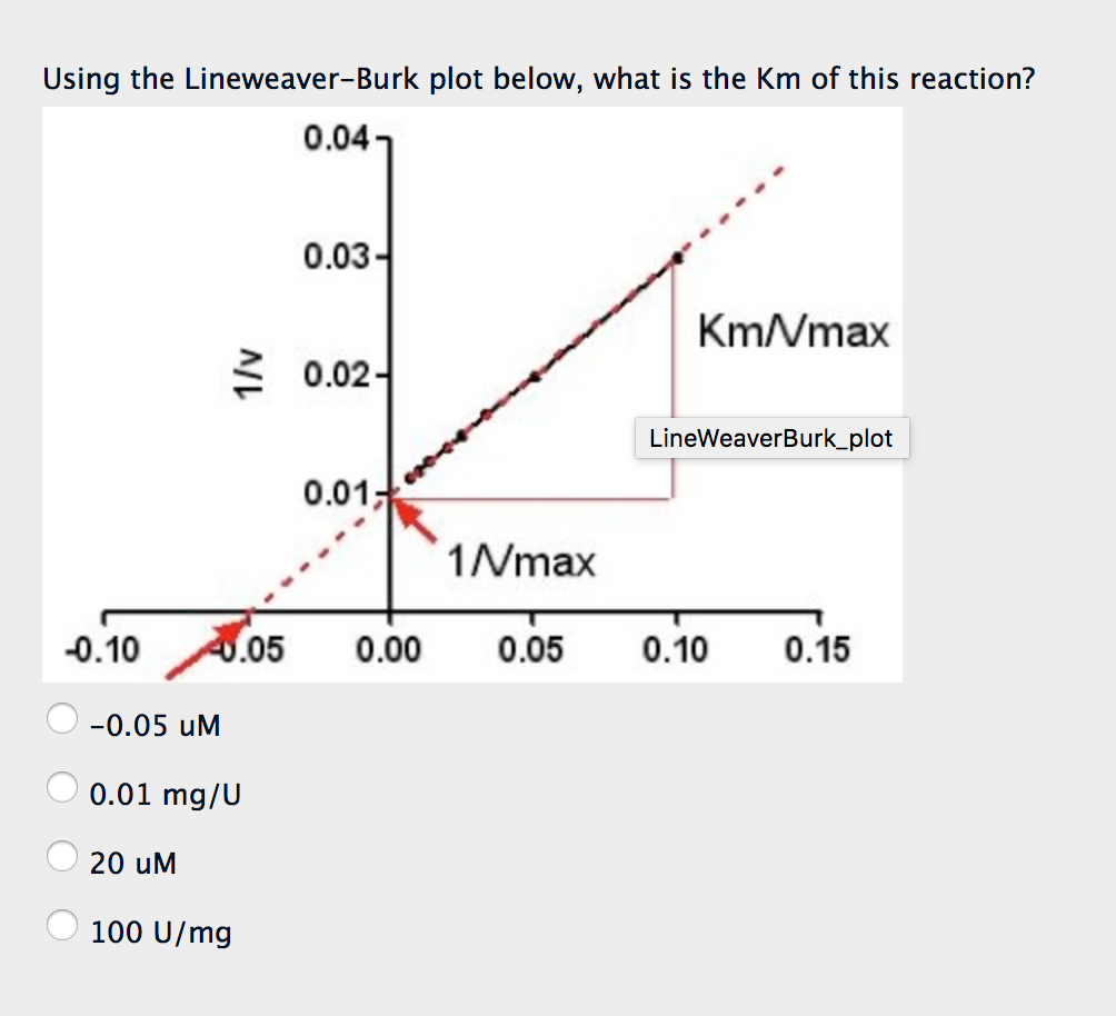
Solved Using the LineweaverBurk plot below, what is the Km
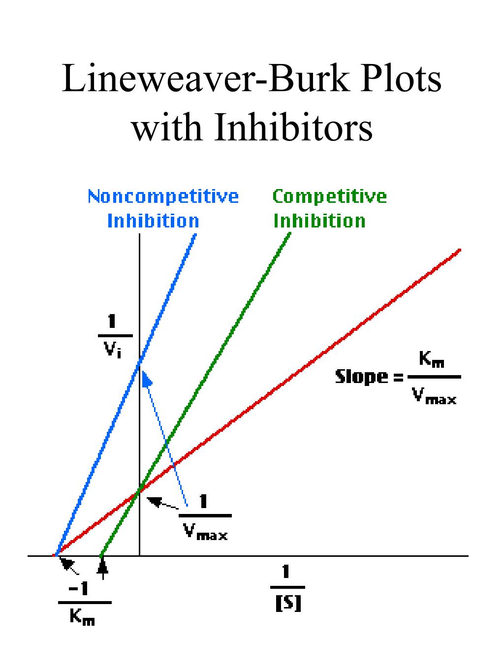
The Lineweaver-Burk plot shows both lines meet the y axis at the same place. In contrast, the following plot shows noncompetitive inhibition. Once again, the regular line is the lower one, whereas the upper line is the inhibited one. The two lines do not share the same y intercept, however. However, they do share the same x intercept.

LineweaverBurk Plot against substrate concentration 2 mM to 10 mM... Download Scientific Diagram
Lineweaver Burk plots show that the Vmax was calculated at 9 nmoles per mg per 30 min, or 1.3 nmoles per pineal per 30 min. From: Serotonin and Behavior, 1973 Add to Mendeley About this page Molecular Aspects of Inhibitor Interaction with PDE4 Siegfried B. Christensen,. Theodore J. Torphy, in Phosphodiesterase Inhibitors, 1996
Lineweaver Burk plot. The data on Xaxis indicate the 1/substrate while... Download Scientific
What Is Lineweaver Burk Plot? A Lineweaver Burk Plot is the graphical representation of the Lineweaver Burk Equation. The plot is used to compare with no inhibitor to identify the effectiveness of the inhibitor. The following describes the Lineweaver Burk plot's components, Substrate Concentration

Lineweaverburk plot of ACE inhibition by different concentrations of... Download Scientific
affect the plots. A comparison between the two graphic representations direct is illustrated here with two "bad" data points (see Fig. 8.16, WWBH). •The same data points are plotted on adjacent Lineweaver-Burk in the left graph of this figure. Two features of the direct linear plot are immediately evident by comparison.

LineweaverBurk plot of the inhibition of nitric oxide synthase... Download Scientific Diagram
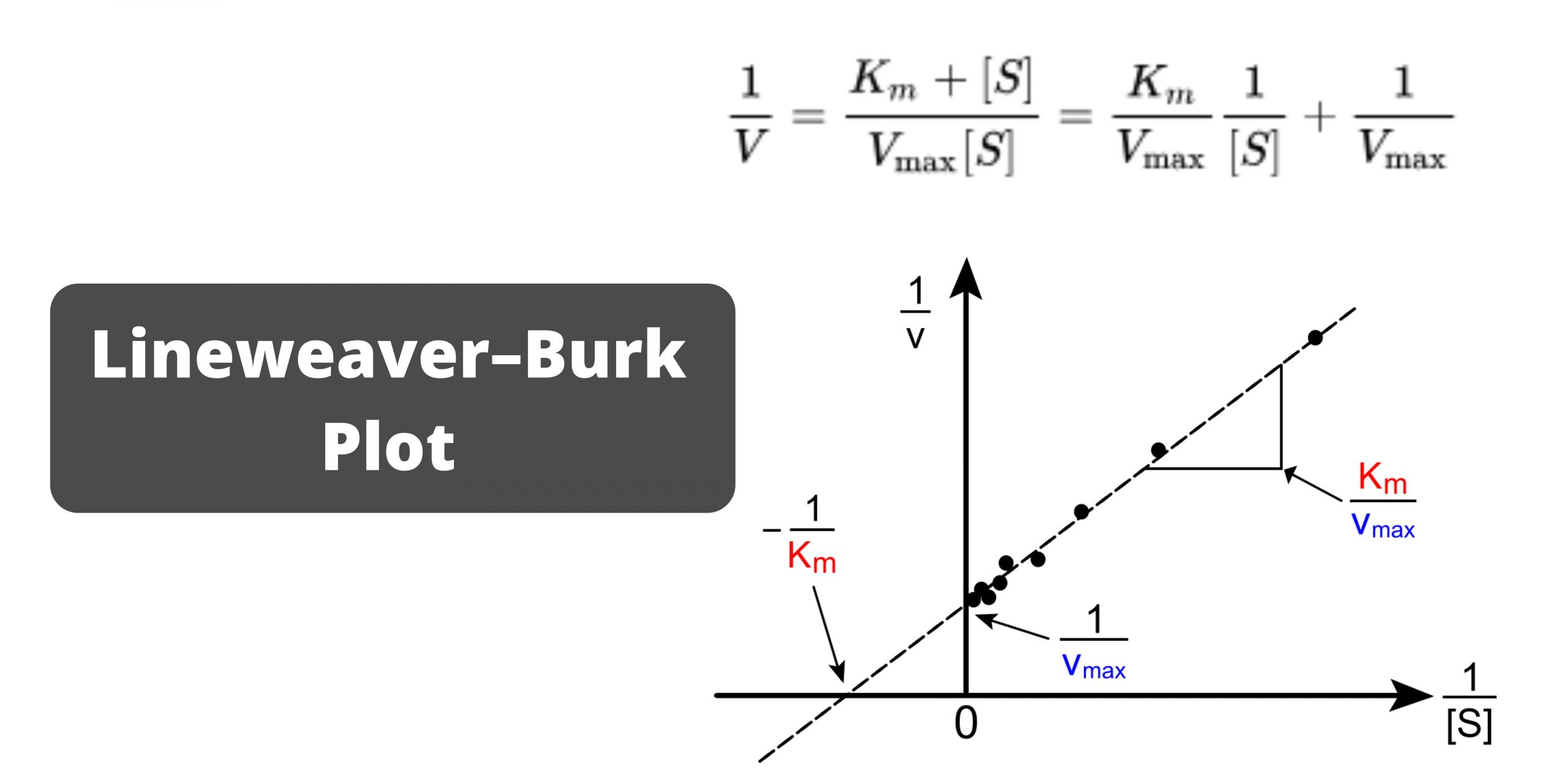
Figure 4.9.1: Line-Weaver Burk Plot. For a Lineweaver-Burk, the manipulation is using the reciprocal of the values of both the velocity and the substrate concentration. The inverted values are then plotted on a graph as 1 / V vs. 1 / [ S ]. Because of these inversions, Lineweaver-Burk plots are commonly referred to as 'double-reciprocal' plots.

Km and Vmax determination by LineweaverBurk plot for free and... Download Scientific Diagram
The Lineweaver-Burk plot was widely used to determine important terms in enzyme kinetics, such as \(K_m\) and \(V_{max}\), before the wide availability of powerful computers and non-linear regression software. The y-intercept of such a graph is equivalent to the inverse of \(V_{max}\); the x-intercept of the graph represents \(−1/K_m\)..

The LineweaverBurk plot for the ACE inhibition pattern of purified... Download Scientific Diagram
The double reciprocal plot (Lineweaver Burk plot) offers a great way to visualize the inhibition. In the presence of I, just Vm will decrease. Therefore, -1/Km, the x-intercept will stay the same, and \(1/V_m\) will get more positive. Therefore the plots will consists of a series of lines intersecting on the x axis, which is the hallmark of.

Create a LineweaverBurk Plot in Excel
The Lineweaver-Burk reciprocal plot presents some problems due to the unequal weighting of errors as illustrated in Figure 1. Figures 1A, B and C show the same data set fit by nonlinear regression to a hyperbola (Figure 1A) compared to fits derived by linear regression using a Lineweaver-Burk plot (Figure 1B) and an Eadie-Hofstee plot (Figure 1C).
How to Make a Lineweaver Burk Plot in Excel (with Easy Steps)
The LibreTexts libraries are Powered by NICE CXone Expert and are supported by the Department of Education Open Textbook Pilot Project, the UC Davis Office of the Provost, the UC Davis Library, the California State University Affordable Learning Solutions Program, and Merlot. We also acknowledge previous National Science Foundation support under grant numbers 1246120, 1525057, and 1413739.

The LineweaverBurk plot, representing reciprocal of initial enzyme... Download Scientific Diagram
The Lineweaver-Burk plot (or double reciprocal plot) is a graphical representation of the Lineweaver-Burk equation of enzyme kinetics, described by Hans Lineweaver and Dean Burk in 1934. This plot is a derivation of the Michaelis-Menten equation and is represented as: Table of Contents

LineweaverBurk plots of reaction velocity versus substrate... Download Scientific Diagram
The Lineweaver Burk plot is a graphical representation of enzyme kinetics. The x-axis is the reciprocal of the substrate concentration, or 1 / [S], and the y-axis is the reciprocal of the reaction velocity, or 1 / V. In this way, the Lineweaver Burk plot is often also called a double reciprocal plot.
LineweaverBurk Plot
To determine the V max from a Lineweaver-Burk plot you would: A. Multiply the reciprocal of the x-axis intercept by -1. B. Multiply the reciprocal of the y-axis intercept by -1. C. Take the reciprocal of the x-axis intercept. D. Take the reciprocal of the y-axis intercept.
